Quantum Computing for Condensed Matter Physics

In this blog post, we aim to encourage the use of quantum computing in quantum many-body-physics. This post is published in the context of the QUICS project, which is a joint project of the Gesellschaft für wissenschaftliche Datenverarbeitung Göttingen, the Leibniz University Hannover, and the Physikalisch-Technische Bundesanstalt. The Federal Ministry of Research, Technology and Space (BMFTR) funds QUICS to provide consultation and low-threshold access to different quantum hardware and software for testing practical use cases, especially for small and medium enterprises. For more information contact us at quics-info@gwdg.de .

To this end, we present the OpenFermion Python library. The main goal of this library is to bridge the gap between quantum algorithm developers and quantum chemists and physicists. In their library, the developers intend to facilitate the development of algorithms for quantum simulations by integrating these groups. With OpenFermion, one can easily describe the Hamiltonian of a molecule or a problem and then use quantum simulators via library plug-ins to study the properties of the quantum system. If you want to know more about this library, please refer to their release paper .

In this blog post, we focus on condensed matter physics, where the properties of states of matter are studied using theoretical models or experiments, such as those involving cold atomic gases. Condensed matter physics includes topics such as high-temperature superconductivity and topological phases of matter. In the past, research in condensed matter theory has led to applications in nanoelectronics and nanostructures, gas sensors, nitrogen-vacancy centers, and more.

The simulation of quantum mechanical systems is one of the earliest proposed applications of quantum computing. The dimension of the Hilbert space of such systems grows exponentially with the system size; thus, simulating a large quantum system using a classical computer is infeasible. Therefore, Feynman proposed the quantum computer in the 1980s as a device to simulate quantum mechanical systems: “Nature isn’t classical and if you want to make a simulation of Nature, you’d better make it quantum mechanical, and by golly it’s a wonderful problem, because it doesn’t look so easy.”

In this tutorial, we study the two phases of the Bose-Hubbard model. We chose this model because it has been widely studied in condensed matter theory, which allows us to compare our results with those in the existing literature. The Bose-Hubbard model describes interacting bosons on a lattice and exhibits a phase transition between the superfluid (SF) and the Mott insulator (MI) phase. The Hamiltonian of the Bose-Hubbard model is \[H = -t\sum\limits_{\langle ij \rangle} a_i^\dagger a_j + \frac{U}{2} \sum\limits_i n_i (n_i -1),\text{.}\] \(\langle ij \rangle\) denotes the summation over neighboring lattice sites, and \(a_i^\dagger\) and \(a_i\) are the bosonic creation and annihilation operators, respectively. \(t\) is the hopping amplitude and \(U\) is the onsite interaction strength. As references for the Bose-Hubbard model, we used the following two papers:

• Quantum phase transition from a superfluid to a Mott insulator in a gas of ultracold atoms
• Collapse and revival of the matter wave field of a Bose–Einstein condensate

The goal of this blog post is to introduce the OpenFermion Python library as a tool for simulating materials via quantum computing. For this, the Hamiltonian of the corresponding system is used. OpenFermion provides functions for specific Hamiltonians, such as bose_hubbard,’ and includes a framework to build operators or Hamiltonians as desired. The library can also be used for quantum chemistry problems, particularly to determine the electronic configuration of molecules. The code is available as a notebook, which is included in our OpenFermion Apptainer container in the directory /opt/notebooks/. Our quantum computing containers can be found here . Later, there will be the possibility of using quantum simulators within the HPC environment provided by the QUICS project.

Study the two phases

First we look at the border cases. In the SF phase, the interaction strength \(U\) is zero. In this case, the many-body wavefunction is delocalized. The inverse participation ratio (IPR) is a measure of localization and is defined as \[IPR = \sum\limits_\alpha \mid\phi_\alpha\mid^4\, ,\] where the sum is over all the Fock basis states \(\alpha\). In an extended/delocalized state, the IPR vanishes. The IPR is non-zero only in a localized state. Therefore, in the SF phase, we expect the IPR to be small. For \(t = 0\), we have the MI phase. Here, the many-body wavefunction is expressed by localized atomic wavefunctions. Therefore, we expect the IPR to be close to \(1\). This is how one can create the Bose-Hubbard Hamiltonian and calculate the IPR with the OpenFermion library:

import numpy as np
from openfermion.hamiltonians import bose_hubbard
from openfermion.linalg import get_sparse_operator, get_ground_state

H = bose_hubbard(
        x_dimension,
        y_dimension,
        tunneling,
        interaction,
        chemical_potential=0.5,
        dipole=0.0,
        periodic=True,)

H_sparse = get_sparse_operator(H, trunc=trunc)
eigenenergy, eigenstate = get_ground_state(H_sparse)

# Calculate the IPR:
IPR_SF = np.sum(np.abs(eigenstate)**4)

Indeed, from this, we obtain \(IPR_{SF} = 0.00139\) and \(IPR_{MI} = 0.99999\). You can try this yourself in the provided Python notebook. For the MI phase, localization alone is insufficient to determine whether the MI phase has been found. It is also necessary to ensure that a gap appears in the excitation spectrum:

from openfermion.linalg import get_gap,
gap = get_gap(H_sparse)
print("Gap in the excitation spectrum: ", gap)

From this, one obtains’ Gap in the excitation spectrum: 0.49999999999998135`, so we have indeed found the MI phase.

Time evolution after a Quench

We now study the time evolution of the Bose-Hubbard model after a quench at time zero. We consider a quench from the SF regime to the MI phase and vice versa. To perform the time evolution of boson operators via OpenFermion, one can use the SFOpenBoson plugin or Strawberry Fields toolbox. To determine the localization over time, we calculated the IPR using the time-dependent state of the system. This is how the time evolution is constructed with OpenFermion:

from sfopenboson.ops import BoseHubbardPropagation
from strawberryfields.ops import *
import strawberryfields as sf

k = 20 # Lie product truncation
for time in total_time:
    H_MI = bose_hubbard(
               x_dimension,
               y_dimension,
               t_MI,
               U_MI,
               chemical_potential=0.5,
               dipole=0.0,
               periodic=True,)
    H_SF = bose_hubbard( # Hamiltonian after quench
               x_dimension,
               y_dimension,
               t_SF,
               U_SF,
               chemical_potential=0.5,
               dipole=0.0,
               periodic=True,)
    prog = sf.Program(n_lattice_sites)
    with prog.context as q:
        Ket(eigenstate_MI) | q
        BoseHubbardPropagation(H_SF, time, k, mode='global') | q
        
    eng = sf.Engine("fock", backend_options={"cutoff_dim": trunc})
    final_state = eng.run(prog).state
    state_vector = final_state.ket()

The time evolution is executed with the function BoseHubbardPropagation using the Lie-product formula and decomposing the unitary operations into a combination of beam splitters, Kerr gates, and phase-space rotations.

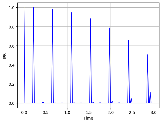
The figure shows the time evolution of the IPR after a quench from the MI regime to the SF phase. It can be seen that the initial MI phase vanishes over time but recurs later. The recurrence of a phase is also shown in the second Bose-Hubbard paper cited above, where they quenched from the SF phase into the MI phase in an experiment with cold atoms in an optical lattice.

As you can see, Hamiltonians can be easily implemented with OpenFermion and their properties can be studied using quantum computing. This can lower the barrier for quantum chemists and physicists to enter quantum computing and solve their problems using quantum computing. There are different models, other than the Bose-Hubbard model, already implemented in the OpenFermion library, such as d-wave models of superconductivity, the Richardson-Gaudin model, or models for the uniform electron gas (jellium). OpenFermion also includes different methods, such as the Hartree-Fock method, Davidson method, and Grassmann wedge product. Therefore, you can try other Hamiltonians or setups in the library. As an outlook, there are different papers studying the electronic structure and ground state of different molecules and models via quantum computing: for example the FeMoco molecule and Cytochrome P450 , \(BeH_2\), \(CH_4\), \(H_2O\), \(HF\) and \(NH_3\) , an \(H_4\) square, an \(H_4\) chain, and the Hubbard model , or uniform electron gas, diamond, and nickel oxide . All of them used the OpenFermion library at least partially in their calculations.